Transfer Learning for Detecting Obfuscated Malware: A Comprehensive Overview

In the ever-evolving landscape of cybersecurity, the detection of obfuscated malware presents a significant challenge. This article delves into a transfer learning model designed to enhance the detection of such malware, detailing the data collection process, system model preparation, and the deep learning (DL) and transfer learning (TL) methodologies employed.

Data Collection and System Model Preparation

The foundation of any effective malware detection system lies in its data. This study utilizes three distinct datasets: MalwareMemoryDump, NF-TON-IoT, and UNSW-NB15. Each dataset serves a unique purpose in evaluating the efficacy of the proposed detection methods.

MalwareMemoryDump Dataset

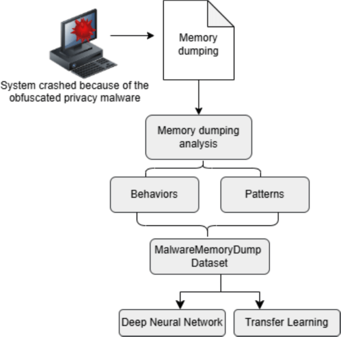
The MalwareMemoryDump dataset is specifically curated to assess the detection capabilities of obfuscated malware through memory analysis. It includes a balanced representation of malware types, such as Trojan Horses, ransomware, and spyware, ensuring a realistic testing environment. The dataset comprises 58,596 records, evenly split between malicious and benign samples, which helps in training robust models.

NF-TON-IoT Dataset

The NF-TON-IoT dataset is an adaptation of the ToN-IoT dataset, focusing on cybersecurity applications within Internet of Things (IoT) environments. It records network traffic as NetFlow records, providing a simplified yet effective representation of network flows. With over 1.3 million data flows, this dataset includes a wide range of attack classifications, making it invaluable for training and evaluating detection models.

UNSW-NB15 Dataset

Developed by the University of New South Wales, the UNSW-NB15 dataset is a benchmark for network intrusion detection systems (NIDS). It encompasses various modern attack methods, including denial of service (DoS) and reconnaissance attacks. With approximately 2.6 million records, this dataset is crucial for understanding real-world cybersecurity threats.

Data Preprocessing

Data preprocessing is a critical step in preparing raw data for machine learning (ML) and deep learning (DL) models. The preprocessing steps include:

1. Handling Missing Values: Using the isnull().sum() function, the dataset is evaluated for completeness, identifying columns with null values for further action.

2. Normalization: The min-max scaling technique is employed to ensure that all features are on a similar scale, which is essential for effective model training. The formula used is:

   [
   D{\text{scaled}} = \frac{D – D{\text{min}}}{D{\text{max}} – D{\text{min}}}
   ]

3. Label Encoding: Categorical labels are converted into numerical form to facilitate model training.

These preprocessing steps ensure that the dataset is clean and ready for model training.

Deep Neural Network (DNN) Model

The initial phase of the model involves training a Deep Neural Network (DNN) using the preprocessed data. DNNs consist of multiple hidden layers that allow for the identification of complex patterns within the data. The architecture includes:

• Input Layer: Receives feature vectors from malware memory dumps.
• Hidden Layers: Perform feature extraction and transformation.
• Output Layer: Generates the final classification outcome, distinguishing between malware and benign samples.

Mathematically, the DNN can be represented as follows:

[
Z^{(l)} = W^{(l)} A^{(l-1)} + b^{(l)}
]

[
A^{(l)} = f(Z^{(l)})
]

where (Z^{(l)}) is the weighted sum of inputs, (W^{(l)}) is the weight matrix, and (A^{(l)}) is the activation output.

Transfer Learning Methodology

Transfer learning is a powerful technique that allows for the application of a pre-trained model to a new but related task. In this study, the pre-trained DNN model serves as the foundation for detecting malware in the target domain.

Transfer Learning Process

1. Base Model Selection: A pre-trained model is selected based on its performance on the source dataset.

2. Freezing Layers: The weights of the pre-trained layers are frozen to retain the learned features, while new layers are added for the target task.

3. Fine-Tuning: The model is fine-tuned using the NF-TON-IoT and UNSW-NB15 datasets, allowing it to adapt to the specific characteristics of the target domain.

The overall optimization objective for transfer learning can be expressed as:

[
L_{\text{total}} = \lambda \cdot L_s + (1 – \lambda) \cdot L_t
]

where (L_s) is the source task loss, (L_t) is the target task loss, and (\lambda) is a weighting factor.

SHAP for Model Interpretability

To enhance the transparency of the model’s predictions, SHapley Additive exPlanations (SHAP) values are employed. SHAP provides insights into how each feature contributes to the model’s predictions, which is particularly valuable in cybersecurity applications. The SHAP value of a feature (x_i) is calculated as follows:

[
\phii = \sum{S \subseteq F \setminus {i}} \frac{|F|!}{|S|!(|F| – |S| – 1)!} \left[ f(S \cup {i}) – f(S) \right]
]

This method allows for a deeper understanding of the model’s decision-making process, facilitating better threat analysis.

Conclusion

The proposed transfer learning model for detecting obfuscated malware demonstrates a robust methodology that combines deep learning techniques with effective data preprocessing and interpretability through SHAP values. By leveraging pre-trained models and fine-tuning them on specific datasets, the model not only enhances detection accuracy but also provides transparency in its predictions. This approach is crucial in the ongoing battle against sophisticated malware threats, ensuring that cybersecurity measures remain effective and adaptive in a rapidly changing digital landscape.